Python:Linear Algebra

Sweeping a Parameter

If you have a system where the coefficients change as a function of some parameter, you will generally need to use a loop to solve and store the solutions. If you have a system where the forcing function (right-side vector) changes, you may be able to solve all at once but generally a loop is the way to go. The following shows example code for sweeping through a parameter, storing values, and then plotting them:

Changing coefficient matrix

Equations

For this example, the equations are:

\( \begin{align} mx-y&=4\\ x+y&=3 \end{align} \)

which means a matrix-based representation is:

\( \begin{align} \begin{bmatrix} m & -1\\1 & 1 \end{bmatrix} \begin{bmatrix} x\\y \end{bmatrix} &= \begin{bmatrix}4\\3 \end{bmatrix} \end{align} \)

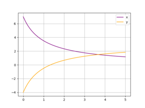
The determinant for the coefficient matrix of this system is \(m+1\) meaning there should be a unique solution for all values of \(m\) other than -1. The code is going to sweep through 50 values of \(m\) between 0 and 5.

Code

Graph of solutions with parameter sweep

import numpy as np
import matplotlib.pyplot as plt

m = np.linspace(0, 5, 50)
x = []
y = []

for k in range(len(m)):
    A = np.array([[m[k], -1], [1, 1]])
    b = np.array([[4], [3]])
    soln = np.linalg.solve(A, b)
    x.append(soln[0][0])
    y.append(soln[1][0])
    
plt.figure(1)
plt.clf()
plt.plot(m, x, color='purple', label='x')
plt.plot(m, y, color='orange', label='y')
plt.grid(1)
plt.legend()

Changing solution vector

Equations

For this example, the equations are:

\( \begin{align} x-y&=p\\ x+y&=3 \end{align} \)

which means a matrix-based representation is:

\( \begin{align} \begin{bmatrix} 1 & -1\\1 & 1 \end{bmatrix} \begin{bmatrix} x\\y \end{bmatrix} &= \begin{bmatrix}p\\3 \end{bmatrix} \end{align} \)

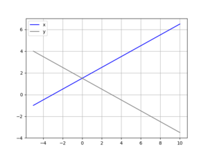
The determinant for the coefficient matrix of this system is 2 meaning there should always be a unique solution. The code is going to sweep through 75 values of \(p\) between -5 and 10.

Code

Graph of solutions with parameter sweep

import numpy as np
import matplotlib.pyplot as plt

p = np.linspace(-5, 10, 75)
x = []
y = []

for k in range(len(p)):
    A = np.array([[1, -1], [1, 1]])
    b = np.array([[p[k]], [3]])
    soln = np.linalg.solve(A, b)
    x.append(soln[0][0])
    y.append(soln[1][0])
    
plt.figure(1)
plt.clf()
plt.plot(p, x, color='blue', label='x')
plt.plot(p, y, color='gray', label='y')
plt.grid(1)
plt.legend()

Multiple solution vectors simultaneously

This method is not recommended for people with limited experience with linear algebra.

Equations

For this example, the equations are:

\( \begin{align} x-y&=p\\ x+y&=3 \end{align} \)

which means a matrix-based representation is:

\( \begin{align} \begin{bmatrix} 1 & -1\\1 & 1 \end{bmatrix} \begin{bmatrix} x\\y \end{bmatrix} &= \begin{bmatrix}p\\3 \end{bmatrix} \end{align} \)

The determinant for the coefficient matrix of this system is 2 meaning there should always be a unique solution. The code is going to solve the system for 75 values of \(p\) between -5 and 10 by setting up a 75-column matrix of solution vectors and then extracting the first row of solutions for \(xa\) and the second row for \(ya\). Note that unlike the above two examples where \(x\) and \(x\) were lists, \(xa\) and \(ya\) are arrays.

Code

import numpy as np
import matplotlib.pyplot as plt

p = np.linspace(-5, 10, 75)
rhs = np.block([[p], [3 + 0 * p]]) # note use of 0*p to get array of correct size!
all_soln = np.linalg.solve(A, rhs)
xa = all_soln[0][:]
ya = all_soln[1][:]