Difference between revisions of "Python:Linear Algebra"
| Line 2: | Line 2: | ||
If you have a system where the coefficients change as a function of some parameter, you will generally need to use a loop to solve and store the solutions. If you have a system where the forcing function (right-side vector) changes, you '''may''' be able to solve all at once but generally a loop is the way to go. The following shows example code for sweeping through a parameter, storing values, and then plotting them: | If you have a system where the coefficients change as a function of some parameter, you will generally need to use a loop to solve and store the solutions. If you have a system where the forcing function (right-side vector) changes, you '''may''' be able to solve all at once but generally a loop is the way to go. The following shows example code for sweeping through a parameter, storing values, and then plotting them: | ||
=== Changing coefficient matrix === | === Changing coefficient matrix === | ||
| − | === Equations === | + | ==== Equations ==== |
For this example, the equations are: | For this example, the equations are: | ||
<center><math> | <center><math> | ||
| Line 49: | Line 49: | ||
=== Changing solution vector === | === Changing solution vector === | ||
| − | === Equations === | + | ==== Equations ==== |
For this example, the equations are: | For this example, the equations are: | ||
<center><math> | <center><math> | ||
Revision as of 23:06, 21 October 2018
Contents
Sweeping a Parameter
If you have a system where the coefficients change as a function of some parameter, you will generally need to use a loop to solve and store the solutions. If you have a system where the forcing function (right-side vector) changes, you may be able to solve all at once but generally a loop is the way to go. The following shows example code for sweeping through a parameter, storing values, and then plotting them:
Changing coefficient matrix
Equations
For this example, the equations are:
which means a matrix-based representation is:
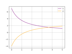
The determinant for the coefficient matrix of this system is \(m+1\) meaning there should be a unique solution for all values of \(m\) other than -1. The code is going to sweep through 50 values of \(m\) between 0 and 5.
Code
import numpy as np
import matplotlib.pyplot as plt

m = np.linspace(0, 5, 50)
x = []
y = []

for k in range(len(m)):
    A = np.array([[m[k], -1], [1, 1]])
    b = np.array([[4], [3]])
    soln = np.linalg.solve(A, b)
    x.append(soln[0][0])
    y.append(soln[1][0])

plt.figure(1)
plt.clf()
plt.plot(m, x, color='purple', label='x')
plt.plot(m, y, color='orange', label='y')
plt.grid(1)
plt.legend()
Changing solution vector
Equations
For this example, the equations are:
which means a matrix-based representation is:
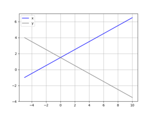
The determinant for the coefficient matrix of this system is 2 meaning there should always be a unique solution. The code is going to sweep through 75 values of \(p\) between -5 and 10.
Code
import numpy as np
import matplotlib.pyplot as plt

p = np.linspace(-5, 10, 75)
x = []
y = []

for k in range(len(p)):
    A = np.array([[1, -1], [1, 1]])
    b = np.array([[p[k]], [3]])
    soln = np.linalg.solve(A, b)
    x.append(soln[0][0])
    y.append(soln[1][0])

plt.figure(1)
plt.clf()
plt.plot(p, x, color='blue', label='x')
plt.plot(p, y, color='gray', label='y')
plt.grid(1)
plt.legend()

