Python:Linear Algebra

General

Solving

To solve Ax=b using linear algebra, be sure that A is a 2D array. b can either be 1D or 2D -- and in fact if 2D it can be a row or a column! Some math packages that solve linear algebra problems would require that b be a 2D column, but not Python. The result x will be the same shape and size as b (that is, 1D, 2D row, or 2D column). Here is an example with b as a 2D column:

A = np.array([[1, 1], [1, -1]])
b = np.array([[3], [4]])
soln = np.linalg.solve(A, b)

for example will create a variable called soln that is:

array([[ 3.5],
       [-0.5]])

Printing solution

Python's format command is picky and will not take arrays. To print out the solutions to the above, for instance, you would need:

print('x: {:f}, y: {:f}'.format(soln[0][0], soln[1][0]))

or perhaps more clearly:

soln_vec = soln[:,0]
print('x: {:f}, y: {:f}'.format(soln_vec[0], soln_vec[0]))

Note that soln[0] will give you an array containing the x value, not just the x value, so while:

print('x: {}, y: {}'.format(soln[0], soln[1]))

works, it is printing out array.

print('x: {}, y: {}'.format(soln[0], soln[1]))

will give an error:

TypeError: unsupported format string passed to numpy.ndarray.__format__

Condition numbers

As noted in Chapra 11.2.2, the base-10 logarithm gives an estimate for how many digits of precision are lost between the number of digits in the coefficients and the number of digits in the solution. Condition numbers based on the 2-norm may be calculated in Python using:

np.linalg.cond(A) # default is based on 2-norm

For information on using other norms to calculate condition numbers, see

help(np.linalg.cond)

and specifically information about the kwarg p. Note that you must use np.inf, not just inf, for the infinity norm.

Sweeping a Parameter

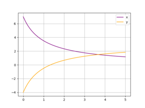
If you have a system where the coefficients change as a function of some parameter, you will generally need to use a loop to solve and store the solutions. If you have a system where the forcing function (right-side vector) changes, you may be able to solve all at once but generally a loop is the way to go. The following shows example code for sweeping through a parameter, storing values, and then plotting them:

Changing coefficient matrix

Equations

For this example, the equations are:

\( \begin{align} mx-y&=4\\ x+y&=3 \end{align} \)

which means a matrix-based representation is:

\( \begin{align} \begin{bmatrix} m & -1\\1 & 1 \end{bmatrix} \begin{bmatrix} x\\y \end{bmatrix} &= \begin{bmatrix}4\\3 \end{bmatrix} \end{align} \)

The determinant for the coefficient matrix of this system is \(m+1\) meaning there should be a unique solution for all values of \(m\) other than -1. The code is going to sweep through 50 values of \(m\) between 0 and 5.

Code

Graph of solutions with parameter sweep

import numpy as np
import matplotlib.pyplot as plt

m = np.linspace(0, 5, 50)
x = []
y = []

for k in range(len(m)):
    A = np.array([[m[k], -1], [1, 1]])
    b = np.array([[4], [3]])
    soln = np.linalg.solve(A, b)
    x.append(soln[0][0])
    y.append(soln[1][0])
    
plt.figure(1)
plt.clf()
plt.plot(m, x, color='purple', label='x')
plt.plot(m, y, color='orange', label='y')
plt.grid(1)
plt.legend()

Changing solution vector

Equations

For this example, the equations are:

\( \begin{align} x-y&=p\\ x+y&=3 \end{align} \)

which means a matrix-based representation is:

\( \begin{align} \begin{bmatrix} 1 & -1\\1 & 1 \end{bmatrix} \begin{bmatrix} x\\y \end{bmatrix} &= \begin{bmatrix}p\\3 \end{bmatrix} \end{align} \)

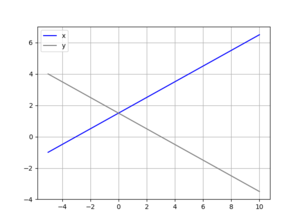
The determinant for the coefficient matrix of this system is 2 meaning there should always be a unique solution. The code is going to sweep through 75 values of \(p\) between -5 and 10.

Code

Graph of solutions with parameter sweep

import numpy as np
import matplotlib.pyplot as plt

p = np.linspace(-5, 10, 75)
x = []
y = []

for k in range(len(p)):
    A = np.array([[1, -1], [1, 1]])
    b = np.array([[p[k]], [3]])
    soln = np.linalg.solve(A, b)
    x.append(soln[0][0])
    y.append(soln[1][0])
    
plt.figure(1)
plt.clf()
plt.plot(p, x, color='blue', label='x')
plt.plot(p, y, color='gray', label='y')
plt.grid(1)
plt.legend()

Multiple solution vectors simultaneously

This method is not recommended for people with limited experience with linear algebra.

Equations

For this example, the equations are:

\( \begin{align} x-y&=p\\ x+y&=3 \end{align} \)

which means a matrix-based representation is:

\( \begin{align} \begin{bmatrix} 1 & -1\\1 & 1 \end{bmatrix} \begin{bmatrix} x\\y \end{bmatrix} &= \begin{bmatrix}p\\3 \end{bmatrix} \end{align} \)

The determinant for the coefficient matrix of this system is 2 meaning there should always be a unique solution. The code is going to solve the system for 75 values of \(p\) between -5 and 10 by setting up a 75-column matrix of solution vectors and then extracting the first row of solutions for \(xa\) and the second row for \(ya\). Note that unlike the above two examples where \(x\) and \(y\) were lists, \(xa\) and \(ya\) are arrays.

Code

import numpy as np
import matplotlib.pyplot as plt

p = np.linspace(-5, 10, 75)
rhs = np.block([[p], [3 + 0 * p]]) # note use of 0*p to get array of correct size!
all_soln = np.linalg.solve(A, rhs)
xa = all_soln[0][:]
ya = all_soln[1][:]